Two Choice Scenarios
Keywords: probability, uncertainty, sampling
Making decisions in uncertain circumstances is an everyday occurrence; Their study ranges across the study of intelligence, natural and artificial. This article explores two idealized problems of making a series of sequential choices to achieve a goal. The correspondence to the real-world is a bit rough and contrived but the solutions are surprising.
Our exploration will illustrate some modes of attack which mathematicians use by applying some heuristics. Most importantly:
What should the solution look like qualitatively? That is, what do we think the solution would look like without doing calculations or detailed math? How does the output change as the problem scales in one or more parameters?
What can we learn from examining specific cases by enumerating successively larger problems (e.g. $n = 1$, $n = 2$, ...)? If necessary, can a program be written which can either exactly find solutions (e.g. by enumerating all possibilities) or approximately (e.g. through Monte Carlo methods)?
What can we learn from examining the beginning and ending boundary cases for different sized problems? If a "best" strategy is to be determined, what do different extreme choices in strategy provide?
Analytical solutions are often discovered and expressed using mathematical induction, that is, we write down a base case (usually a solution that involves a boundary condition) plus an inductive step (taking a statement that is true for N and showing that it is true for $n+1$, or its reverse).
Sequential choice problems that are finite and stopping after the accumulation of information from preceding stages may often be solved using backward induction. We stop at stage $T$ (sometimes called the "horizon") which implies that an optimal rule applies at stages $T-1$, $T-2$, etc.
Our first problem is very simple and derives a useful result using backward induction. Our second problem is a bit more difficult. We will explore specific cases in two different ways before embarking on a method to achieve a very surprising and delightful analytical solution.
Fair selection from a sequence of unknown duration
Our first problem: imagine that you are running a sweepstakes with rules that are like those for many product promotions ("No purchase required!"). You want to be fair, giving an even chance of winning to all entrants. The submitted entries arrive over an extended time period, each in the form of sealed envelopes. You want to announce the winner as soon as possible after the deadline. There are so many entries that it is impractical to create a big barrel that contains all the envelopes for choosing one at random.
You are going to be presented with an unknown (to you) number of envelopes, one at a time. You are told that the current envelope that is being presented to you is either the last one or not the last one. You may keep at most one envelope - if you choose to keep the envelope that is being presented to you then you must destroy the current envelope in your possession. When you make your final selection, the process stops.
Your task is to devise a strategy (or "policy") that will allow you to pick any envelope with even odds (the probability of picking any envelope will be exactly $\frac{1}{N}$, where $n$ is the final count of envelopes).
If you stop the process before the last envelope arrives then something goes very wrong. It is impossible to give the unknown number of remaining envelopes a fair shot if you end the process before the last envelope is presented.
So, until you no longer have any envelopes, each round consists of a single envelope that is presented to you and your choice of one of two actions:
- Keep the envelope you already have and destroy the newly presented envelope; or
- Destroy the envelope you already have and keep the new envelope;
Using backward induction, we focus on the final round and the immediately previous round, where each round is numbered sequentially by $k$ from 1 to $n$. This is our backward inductive solution strategy.
Final ($k=N$):
- To be fair to the very last envelope (the $k$th envelope) that is presented, it should be picked with probability = $\frac{1}{N}$. This is a very useful boundary condition.
- The envelope that is currently at hand is one of the previous $k-1$ envelopes. That envelope is picked with probability = $\frac{N-1}{N}$.
- Therefore, the current envelope at hand has been chosen over the $k-1$ rounds in such a way that each of the preceding envelopes had a fair chance of getting to the final round.
Next to Final ($k = N-1$):
- The probability of picking the $k$th envelope in the next to final round must be equal to a value $P$ such that $P$ * the probability of it being picked in the last round is equal to $\frac{1}{N}$. If $P$ is $\frac{1}{N-1}$ then indeed the final probability is $\frac{1}{N}$.
This indicates that at each round $k$ that the probability of picking the presented envelope should be $\frac{1}{k}$. The initial boundary condition, $k=1$, is fulfilled automatically. This strategy is completely independent of the total number of rounds, $n$.
This solution is very satisfying. Without knowing the total number of envelopes that will be presented we can still implement a policy that is entirely fair to every entrant, even if we can at most keep one envelope at the end of each round.
An optimal sample / stopping point problem
Our second problem is a bit like the process of dating different people before settling down. With each person that you date, you learn a bit about what you find attractive (and perhaps what makes you attractive) and what makes a "perfect match".
An idealized version of the problem goes like this. You have in front of you a set of $n$ identical envelopes that are sealed and have been shuffled into a random order with each possible ordering being equally likely. Each envelope contains a piece of paper with a number that is the unique value (say, money that could be awarded) for choosing that envelope instead of all others. Nothing else is known about the distribution of the values within the envelopes.
Your task is to open one envelope at a time and to make a choice whether to discard the contained number or to keep the number contained in the envelope and thereby end the process. All decisions are final. You win the money only if you select the envelope that contains the highest number. No credit for second (or third or ...) best.
A strategy (a "policy") must be devised and followed which maximizes the odds of your selecting the best envelope. As you open envelopes (up to and including when you make your selection) you learn something about the range and distribution of contained values. This is a kind of sampling, of course.
A more formal statement of this problem comes from a very entertaining article by Thomas Ferguson[1] where "secretarial applicants" takes the place of "envelopes":
- There is one secretarial position available.
- There are $n$ applicants for the position; $n$ is known.
- It is assumed you can rank the applicants linearly from best to worst without ties.
- The applicants are interviewed sequentially in a random order with each of the n! orderings being equally likely.
- As each applicant is being interviewed, you must either accept the applicant for the position and end the decision problem or reject the applicant and interview the next one if any.
- The decision to accept or reject an applicant must be based only on the relative ranks of the applicants interviewed so far.
- An applicant once rejected cannot later be recalled.
- Your objective is to select the best of the applicants; that is, you win 1 if you select the best, and 0 otherwise.
Devising a policy entails using what we learn each time an envelope is opened, right up to the time that we select an envelope.
The qualitative structure of the policy is where we must start. My claim is that no matter what we learn up to a given point in the sequence, that the best decision that we can make is to pick the first envelope that meets or exceeds some estimate of the greatest value expected for all envelopes. A "learning phase" attempts to create a good estimate of this greatest value expected by calculating some statistic from the observed values. An "acting phase" opens envelopes until an envelope is found that fulfills our criterion or until we run out of envelopes.
There must be some point in the sequence where we stop our learning phase and switch to our acting phase. But what is the point where learning stops and acting begins? And how do we justify this qualitative structure for a policy?
We can explore the characteristics of the learning phase:
We could choose to learn nothing and merely pick a number $k$ at random and select that envelope. (No learning from our opening and immediately discarding envelopes 1 to $k$ - 1). The chance of this being the best envelope is $\frac{1}{n}$. This represents the worst we can do with the only virtue that it requires no thinking on our part. Not very compelling, I'm afraid.
As we open each envelope, we could try to estimate what may be the largest value from what we have seen. Unfortunately, not only do we not know what the underlying distribution is, we do not even know its form for parametric learning. We can calculate sample moments, the low value seen, the high value seen, the current number of seen envelopes and the number of remaining envelopes. However, the only things that we know for sure is that
- If the highest value envelope is one that we have discarded, then we have already lost; and
- any envelopes that have not yet been seen but have lower values should not be picked (and if we run out of envelopes then we have lost).
The decision function at both extrema is clear - we should not select the first envelope because we have not yet learned anything. And if we do not decide until we get to the end, then we must take the last. In both cases, the chance of selecting the best envelope is $\frac{1}{n}$.
We may open the first $k$ envelopes and derive statistics from their values where $k$ is determined as a function of $n$. The only useful (suffient) statistic is the maximum value of the $k$ observed values. We then use that value as an estimate for the maximum value of all of the $n$ values. This provides a basis for a rational action phase: Pick the envelope with the first value that is greater than this number or as an alternative, pick the $j$th envelope that is greater than this number. While interesting to contemplate (and possibly simulate through experiments) there seems to be little justification for any value of $j$ > 1.
We start by investigating the problem empirically by looking at successively larger problems. Then we will develop an analytical solution.
We represent $n$ envelopes as an array of the same length where each element of the array is an integer provided by permuting the values of 1 to $n$.
We enumerate the sizes $n = 1$, $n = 2$, ... and then try to see a pattern. The first non-trivial case is for $n = 3$.
We permute the possibities as $n!$ rows in a table. Suppose for $n = 3$ we choose to learn with $j = 1$. Then we can see that we would win half of the time. This is much better than if we chose at random (winning $1/3$ the time). Encouraging but much too small of an experiment to give us much confidence.
| 1st | 2nd | 3rd | Outcome |
|---|---|---|---|
| 1 | 2 | 3 | lose |
| 1 | 3 | 2 | win! |
| 2 | 1 | 3 | win! |
| 2 | 3 | 1 | win! |
| 3 | 1 | 2 | lose |
| 3 | 2 | 1 | lose |
The number of permutations of an array of length is $n!$. Recall that factorial values grow prodigiously.
- $3! = 6$
- $4! = 24$
- $5! = 120$
- $6! = 720$
- $7! = 5040$
- $8! = 40320$
- $9! = 362880$
- $10! = 3,628,800$
- …
- $15! = 1,307,674,368,000$
Obviously, attempting to exhaustively test all permutations for $n > 10$ isn't a good idea.
We can roll up our sleeves and work through the math and then run a simulation where we simulate many runs with a large $n$.
Formal Analysis
The best envelope can occur in any of the positions 1 .. $n$. We have three cases:
- The best can occur as one of the envelopes opened during the learning phase. If this happens then we will definitely lose.
- The best can occur during the action phase and before any occurrence of a value that is greater than the greatest value seen during the learning phase. If this happens then we will win.
- The best can occur during the action phase but after a value that is greater than the greatest value seen during the learning phase. If this happens then we will lose.
Let's proceed by labeling a the positions of two envelopes as $j$ and $k$, each ranging from 1 to $n$.
Let $j$ be the position of the best envelope and let $k$ be the position of the last envelope in the learning phase. From the three cases above we know:
- If $j \le k$ then we lose.
- If $j$ is to be selected and it wins then the best of the first $j-1$ candidates (the ones preceding $j$) must have been seen in the learning phase (has position somewhere from 1 to $k$). The probability of success is then the ratio of the number of positions in the learning phase ($k$) to the number of positions prior to our best at $j$ (that number being $j-1$).
We have then:
Each position has a probability of being the best equal to $\frac{1}{n}$. So for a given total number of envelopes $n$ and number of envelopes in the learning phase $k$ we have a probability of success:
Taking the limit as $n$ becomes large:
Finally, a little calculus. We want to find the maximum value for $Pr_n(k)$. Substituting x = k/n and differentiating we find:
Setting this to zero allows us to determine the value of x which corresponds to the maximum probability. Thus, $x = \frac{1}{e}$.
(After confirming, of course, that the second derivative is negative!)
For the policy that we have adopted, the optimal learning phase sample size is the closest value of $k$ such that $\frac{k}{n} \approxeq \frac{1}{e} \approxeq 36.79$%. Surprisingly, the resulting chance of success is also $\approxeq \frac{1}{e} \approxeq 36.79$%!
Simulation using Julia
Below I provide a short program written in Julia to simulate for a given value of $n$ the outcome of a large number of trials ($iters$) across the range of $k$ from 1 to $n$.
The Julia code below also includes functions to compute a few values for factorial and Heap's algorithm for enumerating all permutations of an array. Neither of these are used for the simulation.
I use the Fisher-Yates shuffle algorithm to generate random permutations. For more information refer to the article that I wrote in this blog about this algorithm.
#= ============================================================================
    ===========================================================================

    Stopping.jl

    Code for Secretary Problem Stopping Rule
    December 8, 2019
    Peter L. Gabel

    ===========================================================================
============================================================================ =#


using Plots
import Plots.PlotMeasures: px, pt
import Plots: plot, plot!

"""
    fact()

Compute a few values for factorial
"""
function fact()
    for i in 3:10
        println((i, factorial(i)))
    end
    println("...")
    println((15, factorial(15)))
end

# fact()

"""
    allPerms(N, fn)

Heap's algorithm

Generates all possible permutations of N elements of an array without
repetition. More efficient than simple recursive algorithms.

Pass in a function that takes each generated permutation as an argument
Note use of @inbounds macro
"""
function allperms(N, fn)
    perm = collect(1:N)
    c = ones(Int, N)
    n = 1
    k = 0
    fn(perm) # call this on first permuation result

    @inbounds while n <= N
        if c[n] < n
            k = ifelse(isodd(n), 1, c[n])
            perm[k], perm[n] = perm[n], perm[k]
            c[n] += 1
            n = 1
            fn(perm) # call this on each subsequent result
        else
            c[n] = 1
            n += 1
        end
    end
    return
end

function justPrintLn(perm)
    println(perm)
end

# allperms(5, justPrintLn)

"""
    shuffle!(array)

FISHER-YATES Shuffle
(sometimes attributed to Knuth or to Durstenfeld)

Because sometimes you need to randomly shuffle an array, eh?
Shuffle is in-place picking a random element from the front and swapping it
with the backmost element not yet selected.

Note use of @inbounds macro
"""
function shuffle!(array)
    currentIndex = length(array)
    @inbounds while 1 != currentIndex
    # Pick an element in remaining part of the array
        randomIndex = Int64(floor(rand() * float(currentIndex))) + 1

    # Swap selected element with the current element.
      # println((currentIndex, randomIndex, array))
        temporaryValue = array[currentIndex]
        array[currentIndex] = array[randomIndex]
        array[randomIndex] = temporaryValue

    # Next
        currentIndex = currentIndex - 1
    end
    return array
end

# shuffle!(collect(1:10))

"""
    testShuffle(len, iters)

Create a random array of length len and test the fairness of the
Fisher-Yates Shuffle by iterating iters times and reporting
the output.
"""
function testShuffle(len, iters)
    acc = zeros(Int64, len)
    acc1 = zeros(Int64, len)
    for i in 1:iters
        perm = shuffle!(collect(1:len))
        acc = acc .+ shuffle!(collect(1:len))
        sort!(perm)
        acc1 = acc1 .+ perm
    end
    return (acc, acc1)
end

# testShuffle(10, 100)

"""
    applyPolicy(array, k)

Use as acceptance threshold the max of first k elements

array is a permutation 1..N
k is the number of elements that are inspected without selection for max
"""
function applyPolicy(array, k)
    learnMax = 0
    max = length(array)
    for i in 1:k
        if array[i] > learnMax
            if learnMax == max # oops. the max is in the learning phase
                return false # "oops"
            end
            learnMax = array[i]
        end
    end
    for i in k + 1:length(array)
        if array[i] == max
            return true # "yea"
        elseif array[i] > learnMax
            return false # "nope"
        end
    end
    return false # "end"
end

"""
    testPolicy(N, k, iters)

invocation of applyPolicy for fixed N, k

N specifies the generation of random permutations of 1..N
k is the number of elements that are inspected without selection for max
iters is the number of trials to be aggregated
"""
function testPolicy(N, k, iters)
    successes = 0
    for i = 1:iters
        if applyPolicy(shuffle!(collect(1:N)), k)
            successes = successes + 1
        end
    end
    return (successes, successes / iters)
end

# testPolicy(100, 37, 1000)

"""
    testPolicies(N, kMin, skip, roundCnt, iters)

invocation of testPolicy for fixed N

N specifies the generation of random permutations of 1..N
kMin is the start number of elements inspected without selection for max
skip is the increment of k between rounds
rounds is the total number of rounds
iters is the number of trials to be aggregated per round

Note that I am scaling by 100 and rounding the elements of xArray to make
its axis ticks integers. For some values of N, kMin and skip this may
not be ideal for display, but it works well with N = 10,000, kMin = 0, and
skip = 100.
"""
function testPolicies(N, kMin, skip, roundCnt, iters)
    kMax = kMin + skip * (roundCnt - 1)
    if kMax > N
        return "kMax too big!"
    end

    xArray = zeros(Int64, roundCnt)
    yArray = zeros(Float64, roundCnt, 2)

    for i in 1:roundCnt
        k = kMin + skip * (i - 1)
        (successes, prop) = testPolicy(N, k, iters)
        x = k / N
        prediction = k == 0 ? 0.0 : -x * log(x)
        println((i, k, x,
            round(prop; digits = 3), round(prediction; digits = 3)))

        #rounds[i] = k # current round
        xArray[i] = round(100 * x) # k/N
        yArray[i, 1] = prop
        yArray[i, 2] = prediction
    end
    println(xArray)
    println(yArray)
    plot(xArray, yArray)
    return (xArray, yArray)
end

# (x, y) = testPolicies(10000, 0, 100, 100, 100000)
# plt = plot(x, y, title = "Policy Test", xlabel = "100 * k / N",
#   labels = ["Success Proportion" "Prediction"],
#   annotation = [(50, 0.1, "N = 10,000; iters = 100,000")], lw = 2)
# savefig(plt, "policy.png")
Results
Below is a graph for a large value of $n$ (10,000) with 100,000 trials ($iters$). The proportion of successes that occur over the trials and the analytic value for each $k$ are the blue and red lines.
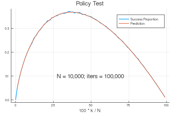
As you can see from the graph of the simulated data, and our calculus, we have confirmed the close correspondence of the simulation and the analytic solution. For the policy that we have adopted, the optimal learning phase sample size is the closest value of $k$ such that $\frac{k}{n} \approxeq \frac{1}{e} \approxeq 36.79$%. Surprisingly, the resulting chance of success is also $\approxeq \frac{1}{e} \approxeq 36.79$%!
Bonus
Below is Heap's algorithm in JavaScript. It may be of interest to the reader to compare this code with the Julia version above.
function permutation(perm) {
  var length = perm.length,
      result = [perm.slice()],
      arr = [],
      i = 1,
      j, p;

  // initialize an array of zeros with same length as perm
  arr.length = length;
  arr.fill(0);

  while (i < length) {
    if (arr[i] < i) {
      j = i % 2 && arr[i];
      p = perm[i];
      perm[i] = perm[j];
      perm[j] = p;
      arr[i]++;
      i = 1;
      result.push(perm.slice());
    } else {
      arr[i] = 0;
      i++;
    }
  }
  return result;
}

function doPerm(n) {
  var arr = [];
  for (var i = 1; i < n+1; i++) {
    arr.push(i);
  }
  return permutation(arr);
}

console.log(permutation([1, 2, 3]));
console.log(doPerm(5), null, '\t')- 1Thomas S. Ferguson, Who Solved the Secretary Problem? Statistical Science, Volume 4, Issue 3, August 1989