Rich Data & Machine Learning

Originally published on Fri, 03/29/2013 - 09:58

Last update on Mon, 12/23/19 - 06:35

A commitment to truth creates a moral imperative that forces you to acknowledge the data and to take the important step of recognizing reality. – M. K. Gandhi

I studied (among many other things) statistics at MIT, where I completed the coursework ordinarily required for a PhD in statistics. Although my interests carried me in other directions than statistics, I worked on a number of truly interesting problems, including applying stochastic methods to representations of social networks to demonstrate some interesting results about rumor contagion.

I have continued to learn and apply state-of-the-art data analysis during my career. It was without irony that I was the development manager for the first versions of Lotus 1-2-3 which for years was the world's leading spreadsheet. Other rich data solutions in my career span fraud detection (a recommended solution by the American Bankers Association), dating and jobs site recommendations and matching, information extraction and analysis for biomedical applications, and more.

This article provides short introductions to a few of the most important concepts of Rich Data and some related techniques. My intent is to provide merely a taste to be savored, not a banquet.

What is Rich Data?

"Rich Data" are decision- and insight-data combined with effective analytic presentations. Rich data leads to both justified actions and the steps to be taken to respond to new information in the future.

The biggest lessons I wish to impart are:

- Rich data is not necessarily big data. The quantity of data is not an indicator of the quality of data. In fact, usually the opposite holds.

• You may be using wrong or poor data features. You have lots of data, but the data does not have the indicators or values that can be used to draw useful conclusions. If you don't have features collected or coded that explain most of the variance of your dependent outcomes, then you are probably in trouble. Sure, you may be able to find some features that proxy for what should have been assembled, but you will probably get a lot of spurious patterns arising.

• You might be poorly preparing your features for a pattern algorithm. You start with potentially rich data and you "simplify" it. For example, text analytics companies are almost always incredibly guilty of putting coherent text through a grinder ("stemming" and "stopping") to create a "bag of words". Now, the average word has about 2.5 separate meanings and most information-laden terms are multi-word expressions. No matter how clever your algorithms, it is still garbage in, garbage out. Yes, linguistics is hard. Its also the only way to make headway. And, if you start with lots of PDF files and aren't smart about extracting text, typically 10-20% will end up being garbled.

- You don't need to do a rich data experiment for anything you can look up in Wikipedia.

• Pattern-based methods are merely methods to apply when you run out of other ways to discover what you need to know. Tycho Brahe, a Dane, collected copious data on the positions of planets. From that, Kepler created the three laws of planetary motion (ellipses with the Sun at one foci, equal areas in equal time, orbital period squared is proportional to the cube of the semi-major axis). Arguably, Kepler was using the "big data" methods of his time. But Newton, in working out the inverse-square law of gravity, used Kepler's laws, not Brahe's data. And Einstein, used his Equivalence Principle which was devised from a thought experiment to work out his theory of gravity and then devised a test involving a single observational experiment (the positions of stars during a solar eclipse).

- There is no free lunch. And there are proofs so don't think otherwise.

• If one algorithm seems to out perform another in one problem setting, it is not because of its overall superiority, it is merely that the algorithm fits the characteristics of the data at hand. This, an informal statement of the No Free Lunch theorem, is not mere folklore. It is a warning that we always need to consider prior biases and models, the data itself, the trade-offs between generalizations and specializations to be made and the way we penalize errors. Marketers may sing the praises of their company's superior algorithms. Beware. Remember that there are bad algorithms and bad approaches out there - but this does not imply there is ever going to be some universal "best" algorithm. Choose wisely.

• Every day I spot something akin to "buy this product or take our on-line course, become a data scientist immediately!" (where have I heard THAT before?) Almost as often, I see articles that unabashedly gush about map-reduce algorithms as a panacea. No. Data science is more about understanding use cases and wise application and interpretation of algorithms than about the algorithms themselves. I would not want to visit a doctor whose knowledge was limited to the inner workings of all of the devices he uses.

- Ugly ducklings are all around us.

• Our analysis is going to be influenced by our assumptions about what an interesting pattern might look like. The "ugly duckling" theorem states that there is no "best" set of features or feature attributes that applies independent of the problem that we are trying to solve. And further, that the assumptions that we make influences the patterns that we see as similar or significant. A very simple example: If I told you that I flipped a coin six times and each time got "heads" you might think that remarkable. If I told you that I flipped a coin and got the sequence H-T-T-H-T-H, you probably would think that ordinary. And yet, each sequence arises with the same probability (1 out of 26).

- 95% confidence means 1 out of 20 times you are dead wrong. Enough said.

- Statistical significance is not the same as true significance.

• We all know the beer and diapers story. It seems compelling - the application of a data mining technique to big data to get a surprising and useful result. The problem in the story is that the application of the technique used (discovery of association rules, most often by applying the "apriori" algorithm) generally creates so many associations that appear to the algorithm to be significant but have no practical value that the approach almost always is to be avoided.

I have had occasion to use a wide variety of approaches over the years, some exciting and some mundane. In this notebook, I have created pages for some technology I would like to share, along with some notes on "The sociology of data." The notes and code on kernel methods and SVMs will be packaged and shared on Github.

Exploratory Data Analysis

-Graphical excellence is that which gives to the viewer the greatest number of ideas in the shortest time with the least ink in the smallest space.- – Edward R. Tufte

Developing and using Know-How.

Developing “Know-How” is a process of accumulating experience and insight around a given subject matter. It involves trial and error, experimentation, exploration and some form of evaluation or review. Progressively, the accumulated knowledge becomes available to the expert in a way that can be shared, redacted and conveyed to someone else.

When people convey ideas, it is often through the use of diagrams, flowcharts, and other visualizations. It is a natural way of describing relationships quickly and efficiently.

Anomalies, tangents, and random thought association

New insights often begin as puzzle pieces that don’t fit. Capturing and pursuing random thoughts, associations, and anomalies can assist in redefining problems and reorganizing ideas that may form paradigm shifts.

Exploring patterns

Often summary statistics are confused with real understanding of the data. Let's look at one extreme example.

Pathological pattern discovery problems can be easily invented by creating datasets as a mixture of randomly points from a small number of distributions. Many of these synthetic sets have striking visualizations when we either limit the creation or project onto two or three dimensions. These datasets serve to benchmark the robustness of pattern recognition algorithms to outliers and different assumptions regarding the number of clusters and cluster shape. For real world data where the number of dimensions is large, it is important to visualize in two or three dimensions different projections of the data to explore if any pathologies may exist.

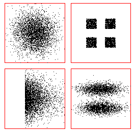
These four data sets have identical mean μ and covariance Σ. Clearly, the ability to create informative clusters depends on the choice of algorithm and parameters. From: Richard O. Duda, Peter E. Hart, and David G. Stork, Pattern Classification. Copyright © 2001 by John Wiley & Sons, Inc.  

Clustering

Cluster algorithms are techniques for assigning items to automatically created groups based on a measurement of similarity between items and groups. Many clustering algorithms exist and again, it is very important to recognize that no algorithm will produce the “best” results for all situations. Some related techniques for unsupervised learning that are not typically thought of as clustering are described in the following section. Additional techniques that incorporate “labelled data” for supervised and active learning are addressed in the next chapter.

Information retrieval applications of clustering have included the organization of documents on the basis of terms that they contain and co-occurring citations, the automated construction of thesauri and lexicons, and in the creation of part of speech and sense taggers. These applications share much in common with exploratory data analysis applications.

There are two major styles of clustering:

- Partitioning. Each example is assigned to one of k partitions (or in the case of fuzzy partitioning, each example is assigned a degree of membership to each partition).

- Hierarchical clustering. Examples are assigned to groups that are organized as a tree structure. Each example is assigned to a leaf and to the nodes that are in the path up to the root node.

The simplest partitioning algorithm is known as k-means. It works as follows. We initialize k distinct values that are initial guesses of the mean values for k distinct partitions. Then iteratively, we assign all examples to the nearest partition (based on some metric) and we recompute the value of each mean. We terminate when the mean values do not change within some tolerance.

The k-means algorithm is sometimes used to seed other algorithms. It has the advantage that it is fast and easy to implement. It has the disadvantage that it may produce poor results if the number of partitions guessed does not match well to the actual structure of the data. Variations include robust methods such as using a median rather than a mean and computing fuzzy membership.

Hierarchical clustering uses a similarity measure to cluster using either a top-down (or divisive) strategy or a bottom-up (or agglomerative) strategy. Divisive strategies start with all examples in a single cluster. A criterion governs how the cluster should be split and how those clusters in turn should be split. Agglomerative clusters start with each example in its own (singleton) cluster. The most similar clusters are merged based on some criterion. Agglomeration continues until either all clusters are merged or another stopping condition is met.

A dendrogram is a particularly useful visualization for hierarchically organized clusters. An example dendrogram appears below.

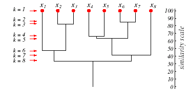
A dendrogram: The vertical axis shows a generalized measure of similarity among clusters. Here, at level 1 all eight points lie in singleton clusters. Points $x_6$ and $x_7$ are the most similar, and are merged at level 2, and so forth. From: Richard O. Duda, Peter E. Hart, and David G. Stork, Pattern Classification. Copyright © 2001 by John Wiley & Sons, Inc.

Many different criteria exist for determining similarity between clusters. These criteria are composed of two things: a measure of similarity between two examples and a strategy for evaluating the similarity between two groups of examples. The measure of similarity is a metric which generally may be thought of as a dot product or, more rigorously, as a Mercer kernel.

Similarity between two groups of examples may be computed in a variety of ways. The most common methods and how they apply to agglomerative clustering follow.

- Single link: At each step the most similar pair of examples not in the same cluster are identified and their containing clusters are merged. Easy to implement, but unsuitable for isolating poorly isolated clusters.

- Complete link: The most dissimilar pairs of examples from different clusters are used to determine cluster similarity. The least dissimilar are merged. This method tends to create small, tightly bound clusters.

- Group average link: The average of all similarity links are used to measure the similarity of clusters. This is a good compromise between the Single link and Complete link methods and performs well.

- Ward’s method: The cluster pair whose merger minimizes the total within-group variance from the centroid is used. This naturally produces a notion of a “center of gravity” for clusters and typically performs well, although it is sensitive to outliers and inhomogenous clusters.

Many variations of these methods exist.

Support Vector Clustering and similar techniques

Support Vector Clustering maps examples in data space to a high dimensional feature space using a Gaussian kernel function

with width parameter q. In feature space the smallest sphere that encloses the image of the data is identified. When mapped back to data space, the sphere forms a set of contours which enclose the data points. These contours form cluster boundaries and may be viewed as a successive set of boundaries for different values of q.

SVC is a variant of a similar method that uses Parzen window estimates for density of the feature space. Other approaches exist. The advantages of these techniques include the ability to cluster over a wide variety of shapes, the ability to control the influence of outliers, and (for some variants) the ability to gracefully deal with overlapping clusters.

Association Rules

Suppose that a large database exists which consists of the SKUs of those items purchased in customer visits to grocery stores. Each transaction may consist of only at most a few dozen SKUs out of a possible set of hundreds of thousands or more. We may ask if the purchase of certain products is predictive of other purchases. For example, we may be able to determine that the purchase of coffee (in this case, we lump all of the SKUs for different brands and packages into one) may be predictive of the purchase of cream. Such a problem is frequently termed “basket analysis.”

The analysis of data for the creation of association rules applies to many business and scientific problems and has been the subject of lively research since the early 1990s. One successful application of the association rule mining algorithm that I performed for CareerBuilder.com is the discovery of patterns of job titles as found within a large corpus of resumes. As might be expected, there are many “career paths” that are shared where one job may lead to others more or less predictably. Discovering and summarizing such patterns from the data led to both well known career paths and a number of surprises.

There are several efficient algorithms (and many variations) that have found broad application. The association rule discovery problem may be formalized as follows. An association rule is an expression X ⇒ Y , where X and Y are sets of items (“itemsets”). The meaning of such rules is interpreted as: Given a database D of transactions, where each transaction T ∈ D is an itemset, X ⇒ Y expresses that whenever T contains X, that T “probably” contains Y. The rule probability or “confidence” expresses the percentage of transactions containing Y that also contain X as compared to all transactions containing X. Thus, we may say, that a customer who buys products x1 and x2 may also buy product y with confidence P.

In addition to confidence, we also speak of the “support” for a particular set or for a rule in a database. The support of a set is the fraction of transactions in D containing that set. The support of a rule X ⇒ Y is defined as the support of X ⋃ Y. We can see that the confidence for a rule may be expressed in terms of support: conf(X ⇒ Y) = supp(X ⋃ Y) / supp(X).

Differences in algorithmic approaches for mining association rules are largely based on differing strategies for traversing the search space of sets of items. One of the most popular algorithms (known as “apriori”) traverses the space in a breadth-first fashion, generating candidate itemsets from known itemsets with at least some minimum support, and then performing counts of those candidate itemsets from the database. The generation of candidates is based on the simple observation that if a given itemset X has support S, then any additional items added to X will never increase the support.

In words, the algorithm works as follows. There are two primary stages: the discovery of all itemsets in D that have some minimum support (“frequent itemsets”), then the analysis of those itemsets for rules that have some minimum confidence. The bulk of the processing and complexity lies in the first stage. The second stage for rule discovery is straightforward – for each frequent itemset x, each subset a is considered for a rule of the form a ⇒ (x – a) . If the rule has minimum confidence then it is output. Variations of this strategy exist for efficiency.

Finding frequent itemsets is based on the creation of candidate itemsets which may be tested for minimum support by counting the number of occurrences within D. The key trick for efficiency is to keep all item identifiers in lexicographic sorted order. Then we can create candidate itemsets that have one more element than those of a previous breadth-first pass by joining existing previous pass frequent itemsets with the condition that a new candidate set x has its first k-2 elements in common with joined itemsets y and z, its k-1 element is the last element of y, its kth element is any element from z, and x must be in lexicographic order. Finally, each subset of length k-1 of the new candidate must be a frequent itemset. This has the effect of pruning the candidates to minimize testing time (say, in the form of database scans) to identify all of the k element itemsets.

Refinements to the association rule discovery problem include methods for creating hierarchical organizations of rules and the creation of rules based on cross-classifications. For example, taxonomies of job titles and job skills can be used as the basis for mining both career trajectories and qualifications through associations and predictive modelling using enhanced hierarchical association rule mining. Refinements to the algorithms focus on alternative search and counting strategies and on the storage of the itemsets.  

Belief Networks

The set of conditional relationships is often expressed as a graph of nodes (events) linked together by directed (causes) and undirected (association) lines. Because of the central role played by Bayes’ theorem in these calculations such graphs are sometimes called Bayesian nets although the more common term used is Belief Networks.

Bayes Theorem says that P(A|B) (the probability of an event A, given event B has occurred) is equal to:

Sometimes in words this is expressed as the “posterior” is equal to the “likelihood” multiplied by the “prior” divided by the “evidence.” The key relationship is the proportionality of the posterior to the likelihood multiplied by the prior.

The power of Belief Networks is that they encode conditional independence. If no path exists between two nodes then the events represented by those nodes are independent. Directed links represent causal relationships, undirected links represent associations. The calculus of Belief Networks is based on the removal or redirection of links associated with a node when information is known about the event that the node represents. This removal and redirection reflects conditional independence.

For example, the example below encodes the features (Fi) are conditionally independent given the disease D.

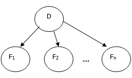
The mathematical expression for this graph is:

Although simple, this kind of encoding of conditionally independent relationships has proven very useful in many applications including text classification and disambiguation of word senses because the calculations are very straightforward and experiments prove that the predictions are typically accurate. It is called “Idiot’s Bayes” or, more graciously, “naïve Bayes.”

A small but interesting Belief Network is illustrated below. It is a directed acyclic graph depicting some possible diseases that could lead to a blue baby. The relationships and the (conditional) probabilities that are not shown were elicited after consultation with an expert pediatrician. This Belief Network is fairly typical – what we wish to conclude (probabilistically) are nodes that are nearer to the top – what we typically observe are nodes nearer to the bottom. Observations may be expressed as probabilities. A Belief Network may then be completed (that is, all remaining probabilities may be determined) through a series of graph manipulations and calculations.

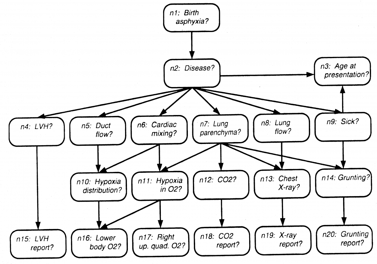
(From Probabilistic Networks and Expert Systems, Cowell, et al).

One use for Belief Networks is modeling risk. Different risk factors may be identified and probabilities may be estimated from experience or from judgment. A new situation that is presented may have known attributes and unknown attributes. Regardless, probabilities of outcomes may be computed.

Belief Network Operations

Belief Networks are defined from models that are elicited from experts or automatically inferred. The inference of network structure is a difficult and interesting area for research and will not be discussed further here. Modeling involves the specification of the relevant variables (generally including both observable and hidden variables), the dependencies between the variables, and the component probabilities for the model.

After a model has been specified it is compiled into a structure more amenable to computation. The graph that encodes the conditional independence relationships constructed by an expert is transformed into an equivalent graph. This involves recasting a directed graph (or a graph with both directed and undirected edges) into an entirely undirected graph. Then edges are added to this graph creating cliques that will enable the joint density of the entire graph to be transformed into a product of factors.

The inference process for a particular situation essentially binds a subset of the variables in the graph and uses the compiled graph to calculate the remainder of the variables through an local update algorithm. I recommend the book by Cowell, et al. as a very complete introduction to Belief Network ideas and algorithms and the book by Pearl as an excellent introduction to Probabilistic Logic.

Bayesian Network References

Cowell, R. G., Dawid, A. P., Lauritzen, S. L. and Spiegelhalter, D. J.. "Probabilistic Networks and Expert Systems". Springer-Verlag. 1999.

Heckerman, David, "A Tutorial on Learning with Bayesian Networks," Technical Report MSR-TR-95-06, Microsoft Research, 1995.

Jensen, F. V. "Bayesian Networks and Decision Graphs". Springer. 2001.

Jordan, M. I. (ed). "Learning in Graphical Models". MIT Press. 1998.

Pearl, Judea, Probabilistic Reasoning in Intelligent Systems: Networks of Plausible Inference, Morgan Kaufmann, San Mateo, CA, 1988.  

Other unsupervised learning techniques

If a dataset has been generated by a process that has an underlying distribution corresponding to a mixture of component densities and if those component densities are described by a set of unknown parameters, then those parameters can be estimated from the data using Bayesian or maximum-likelihood techniques.